NNESMO Session 1 - The basics: 0-D and 1-D models

Prof Jeroen van Hunen

Department of Earth Sciences

Durham University

Practical 1, Part 1: Modelling an Emptying Bathtub
Practical 1, Part 2: Radioactive Decay
Practical 1, Part 3: One-dimensional diffusion
Practical 1, Part 4: Numerical stability
Practical 1, Part 5: Cooling of the Earth (ADVANCED)

Practical 1, Part 1: Modelling an Emptying Bathtub

1.1) Download the file bath.m, and open it in Matlab. Study it briefly, and run the code to see what it does. Make sure you understand what the code is doing.

1.2) Add the analytical solution from the lecture notes to the code and plot.

1.3) How does the numerical model perform for the emptying bath?

1.4) How does the size of the timestep affect your results?

Practical 1, Part 2: Radioactive Decay

Uranium 235 ( ) decays to Lead 207 ( $^{207}Pb$ ), with a half-life $\tau=704$ Myrs. In other words, in 704 Myrs, half of the available $^{235}U$ decays to $^{207}Pb$ . More generally, each unit of time (say each million years) a constant fraction of $^{235}U$ decays to $^{207}Pb$ . The removal of $^{235}U$ (to produce $^{207}Pb$ ) is therefore directly proportional to the available $^{235}U$ itself (check this for yourself!). Let’s simplify notation and call $^{235}U$ simply $N$ . Mathematically, this radioactive decay is then written as:

, with $\lambda$ being the ‘decay constant’.

NOTE: An equation like this one, containing a variable and its derivative, is called a differential equation (henceforth referred to as DE) It nicely describes the physics of (in this case) radioactive decay, but it doesn’t provide an immediate solution for the unknown variable ; we have to solve it first. In some cases, including this one, it is possible to solve the DE analytically — in other cases, a numerical approximation must be used.

Quantities (or rather concentrations) of and $^{207}Pb$ are usually measured with respect to the concentration of a stable isotope of the daughter element, in this case $^{204}Pb$ . At the start of Earth’s life at 4.567 Ga, the concentrations in the mantle of $^{207}Pb$ and $^{235}U$ relative to $^{204}Pb$ were $\frac{^{207}Pb}{^{204}Pb} = 10.294$ and $\frac{^{235}U}{^{204}Pb} = 5.5$ .

1.5) The analytical solution to the DE for radioactive decay is given by . What is the physical meaning of $N_0$ ?

1.6) The relationship between the decay constant and the half-life $\tau$ can be calculated using the analytical solution. Given that the half-life is the time when half of the original radionuclide remains, find $\lambda$ as a function of $\tau$ . What are the units of $\lambda$ ?

1.7) Before programming a numerical model, we first need to translate a (geological?) model into a numerical model. Try to answer the following questions:

What is/are the key mathematical equation(s) we need to solve?
Are there any constants you will need to know? Can you look them up or estimate them?
What will the model look like at time zero? This is the initial condition.
Roughly for how much (model) time will you need to run our model for?

1.8) Rewrite the differential equation in a Forward Euler finite difference format. Rearrange the equation such that the unknown new quantity of $N$ appears on the lefthand side and all known quantities appear on the righthand side of the equation.

1.9) Finally, write the Matlab script to calculate the radioactive decay of and the growth of $^{207}Pb$ in a closed $^{235}U-^{207}Pb$ system from the origin of the Earth to the present day using a Forward Euler method. Build your code in a logical and structured way: set up the sections you think you’ll need, then fill them in one at a time, testing as you go. Plot your results and check that they behave the way you expect. Hint: Rather than referring to ‘old’ and ‘new’ solutions, it is easier to use a timestep counter it, so that the ‘new’ solution refers to the value at timestep it and the ‘old’ solution refers to the value at timestep it-1.

1.10) Add the analytical solutions for both and $^{207}Pb$ to your code, and modify your plots to show the numerical and analytical solutions for both $^{235}U$ and $^{207}Pb$ . How do the numerical solutions compare to the analytical ones?

1.11) Try different timesteps to check that the numerical solution approaches the analytical one for decreasing timesteps. This is called a ‘resolution test’.

1.12) Repeat steps 1.8 to 1.11 for the Backward Euler method and add it to your existing code. How do the numerical and analytical solutions compare now?

1.13) Repeat steps 1.8 to 1.11 for the Crank-Nicholson method and add it to your existing code.

1.14) Calculate the error between the analytical and numerical solutions for for each of the three methods. Add a third section to your plot showing the error through time. Which of the three methods has the smallest error for a given size timestep and why?

Practical 1, Part 3: One-dimensional diffusion

$\frac{\partial T}{\partial t}=\kappa \frac{\partial^2T}{\partial z^2}$

Next, we will familiarize ourselves with the case in which with a variable (in this case temperature) that changes its value not only through time, but also with location. The 1-D heat diffusion equation is given by , where the partial derivative symbol $\partial$ indicates that in the equation $T$ has derivatives to more than one variable (in this case to time $t$ and depth $z$ ). A differential equation such as this one is therefore called a partial differential equation (PDE), and, in contrast, the DEs that we saw before (with derivatives to only one variable) are usually referred to as ‘ordinary differential equations, ODEs).

In this exercise, we will solve the heat diffusion equation for a situation of a cooling oceanic lithosphere: a hot column of mantle material (with temperature C) is emplaced at a mid-ocean ridge, where it suddenly will be in contact with cold ocean water. This column will start cooling from above.

1.15) Sketch (on paper) this temperature distribution as a function of depth $z$ for time $t=0$ . This temperature distribution will be a good initial condition for our modelling exercise.

1.16) Our modelling domain will be the column of mantle material extending to, say, 300 km depth. We already have a governing equation (the heat diffusion equation described above) and an initial condition. To obtain a unique solution, we need to provide boundary conditions at the boundaries (i.e. end points) of the one-dimensional domain, e.g. a fixed temperature, that apply at every time step at the ends of our domain. What would be good boundary conditions for the temperature at $z=0$ and $z=300$ km?

1.17) What does the forward-Euler finite difference form of the diffusion equation look like?

1.18) Suppose we have a system, in which the mantle column is described by just 5 grid points (i.e. ). At the boundaries ( $i=1$ and $i=5$ ) boundary conditions apply, and at the remaining, interior points, the above finite difference equation applies. Write out (again on paper, not in Matlab) for each point $i$ the equation that calculates the temperature at the new time step $T_i^n$ , where $i$ refers to the spatial dimension and $n$ to the time step. If the old solution $T_i^{n-1}$ is known for all $i$ , (and $\kappa$ , $\Delta t$ , and $\Delta z$ are all known as well), we then have all the necessary information to calculate all $T_i^n$ . Perform this calculation manually for this 5-point system for one time step. Assume the first solution to be the initial condition you obtained in 1.15, and assume $\kappa =10^{-6} m^2$ s, $\Delta t=5$ Myr, $\Delta z =75$ km. Note that different units of time and space are used here. Draw this solution onto the schematic plot of the initial condition. Now apply a second time step and again draw the solution to the plot.

1.19) Now copy the Matlab template heat1d.m, and add the missing functions. Run the code, and check how well the numerical solution corresponds to the analytical one.

If time permits, continue with the following exercise.

1.20) We will define it thermal lithosphere as mantle material cooler than C, and want to calculate how thick is the lithosphere as a function of its age. Add to your code a function that calculates the depth for which $T=1200^o$ C, store this information in a time array, and plot it after the time looping has finished. The easiest method is probably to first work out the shallowest grid point for which $T>1200^o$”> C. For a smoother (and more accurate) solution, linearly interpolate between the grid points on either side of the lithosphere lower boundary to find the exact depth for which <img decoding= C.

Practical 1, Part 4: Numerical stability

1.21) Test the time step stability criterion for the radioactive decay problem. Open your radioactive decay code again, increase the total model time to 100 Gyrs, and empirically test which timesteps are stable or instable for the FE, BE, and CN timestepping methods. Calculate the maximum stable timestep for FE using the lecture notes, and compare it to your emperical-found maximum stable timestep.

1.22) Run the heat diffusion code multiple times with larger and smaller time steps, and larger and smaller number of grid points. Do you encounter unstable or unphysical solutions? Also in this case, BE and CN would result in unconditionally stable solutions, but solving a spatially one-dimensional (or more generally more-dimensional) problems with BE or CN is more complex that the one without any spatial variation (such as our radioactive decay problem), and will be discussed later.

Practical 1, Part 5: Cooling of the Earth (ADVANCED)

The (potential) temperature T of the Earth’s upper mantle today is about , but heat released from accretion of the Earth and differentiation into a core-mantle layered system probably heated the early internal Earth to several $100 K$ hotter than that. Since then, radio-active decay added (and still adds) another significant amount of heat, while the only way for the Earth to lose its heat is through its surface. A simple heat balance for the Earth states that the difference between the total radioactive heat source for the whole Earth, $H$ , and the total heat sink for the Earth, $Q$ , (surface heat flow) leads to cooling (or heating) of the Earth. Mathematically, this can be expressed as: $C\frac{dT}{dt} = H(t) - Q(t)$ , with $C=7\times10^{27}$ $JK^{-1}$ the Earth’s total heat capacity. $T$ , $H$ , and $Q$ generally are all functions of time $t$ .

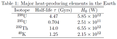
1.23) The following table lists the 4 most important decay systems for the Earth’s thermal history, using , with $\lambda$ related to the half-life of a decay system as $\lambda=\ln(2)/\tau$ :

Give an analytical expression for the total H(t) for the whole Earth through time. depends on past surface tectonics, which is less well known: today, plate tectonics with plate speeds of 5-10 cm/yr is responsible for $Q=36$ TW, but whether this value is valid for the Earth’s whole history is unclear. Maybe plate tectonics was slower or faster (or even non-existent) in the past. To start with, we will assume that $Q$ was always 36 TW. Note that since $\frac{dT}{dt}$ is not dependent on $T$ , this not a d.e., and can be easily solved analytically, provided $H$ and $Q$ are simple functions of time.

1.24) Construct a finite difference code to calculate the thermal history of the Earth. Go through all the necessary steps to arrive at a numerical model:

What is the governing equation for this problem?
Discuss the initial condition.
How to discretise your problem?
Write the numerical code.
Hint: can be chosen to be either today (in which case time runs backward) or at the time of Earth’s accretion (so that time runs forward). Note that this forward or reverse sense of time has nothing to do with Forward or Backward Euler timestepping.

1.25) Plot the resulting temperature as a function of time. According to this (simple) model, did the Earth always cool down over time?

1.26) Test the code with a convergence test, and compare results with those of your colleagues.

If time permits, implement the following adaptations.

1.27) The Urey ratio is defined as the present-day ratio of $H/Q$ , and is thought to be anywhere between $Ur = 0.2$ and $0.5$ . Vary $Ur$ by multiplying the total heat production with a constant prefactor, and explore how that affects the Earth’s thermal evolution. Plot multiple $Ur$ results in a single plot.